Vavuq

A post processor to assess quality of numerical simulations

Introduction

VAVUQ (Verification And Validation and Uncertainty Quantification) can be used as a general purpose program for verification, validation, and uncertainty quantification. The motivation for the creation of and continued development of the program is to provide a cost effective and easy way to assess the quality of computational approximations. The hope is that the methods used in this program can be applied to fields such as civil engineering where they are currently often underutilized. This code was created through efforts from Bombardelli's group and Dr. Bill Fleenor at the University of California Davis. The creators belong to the Civil & Environmental Engineering (CEE) Department, the Center for Watershed Sciences (CWS), and the Delta Solution Team (DST). The main code development is headed by Kaveh Zamani and James E. Courtney.

Download

Download the code.

The source code to Vavuq, its samples, and this website are available on GitHub.

The following is a self-extracting 7-ZIP archive which contains a 64 bit Windows executable of VAVUQ along with example files. The repository code may be more up to date than the executable.

Filename	Size	Last Modified	SHA-256
VAVUQ.exe	63.9 MB	2016-07-06	7B9376925A6EA93D96254EA4AC3A65BE460AC23ADA92E4FE771E3CC337AB7C79

Using Vavuq

1. Introduction

VAVUQ is developed by the Civil and Environmental Engineering department at the University of California Davis (UCD). This software facilitates validation, verification, and uncertainty quantification studies for numerical simulations. The verification and uncertainty quantification components require refinements of a numerical simulation. The validation component requires numerical simulation results and benchmark values. VAVUQ was created as part of efforts at UCD to increase the consistency of quality applications of numerical models to water resources engineering scenarios.

This section discusses the capabilities and general philosophy of VAVUQ. Information specific to VAVUQ is provided in this manual and the online wiki located at the project webpage.

Contents

• General Philosophy
• Capabilities Overview
• Documentation
• Manual Overview

Program General Philosophy

VAVUQ integrates various cross-platform, free, and open-source software libraries to facilitate the application of validation, verification, and uncertainty quantification of numerical codes. The VAVUQ software package consists of a graphical user interface (GUI), data visualization components, interpolation libraries, statistical tools, and tools to read various input file types.

Four quality control components are contained in VAVUQ: (1) Validation statistical metrics that can be used to compare mathematical models to observational data; (2) Calculation of the observed order of accuracy for numerical simulations with unknown exact solutions; (3) Calculation of the observed order of accuracy for numerical simulations where an exact solution (or dense mesh solution or spectral solution) can be obtained; (4) Uncertainty Quantification for determining numerical discretization error bands for chosen degrees of confidence. In addition, the system provides visualization options for each component. Data can be saved in a spreadsheet format for grid interpolations and calculations or as text for normalized calculations and other text-based output.

VAVUQ currently supports comparisons of 2D numerical approximations for both structured and unstructured meshes. Future releases of the program will support comparisons of 3D numerical approximations.

Overview of the Program Capabilities

VAVUQ is designed to perform quality control calculations for numerical simulations. The major capabilities of VAVUQ are described in the following portion of this section.

User Interface

A graphical user interface (GUI) allows user interaction with VAVUQ. The user interface is designed with the goal of facilitating software operation and promoting efficiency. The following functions are provided with the interface:

• Method selections
• Interpolation selections
• Data visualization
• Input file selection
• Displayed output from the methods
• Selection of specific spatial regions to apply the verification methods
• Output saving options
• Help options

VAVUQ Components

Validation. This component of VAVUQ is intended for comparing numerical simulation data to observed data. Comparisons are made with different statistical calculations. Depending on the modeled system, some of the calculated metrics may be more appropriate than others. Calculations can be made with a list consisting of observed data and another list corresponding to numerical approximations of the system the observed data was obtained from.

Solution Verification. This component of VAVUQ is capable of approximating the observed order of accuracy from three numerical simulations. The observed order of accuracy is approximated by determining the spatial discretization of each simulation and the differences between each refinement. The discretizations of the different simulations are determined with VAVUQ. Simulations with nodes that do not overlap can be compared with different interpolation routines. Three equations for truncation error are used to produce an expression that is solved for the observed order of accuracy. The expression is approximated with a direct substitution iterative procedure.

Code Verification. This component of VAVUQ approximates the observed order of accuracy from two numerical simulations and an exact solution. The calculation is made by relating two expressions of truncation error to solve for the observed order of accuracy. The assumed exact solution can be from an analytical solution, a dense mesh, or results from the method of manufactured solutions. The verification option requires the user to input three numerical simulations so that the observed order of accuracy can be calculated twice. This allows the user to assess whether the calculations are consistent.

Uncertainty Quantification. This component of VAVUQ is capable of approximating error bands from numerical approximations. This is achieved by determining the observed order of accuracy and then applying the grid convergence index with a specified safety factor. Different safety factors can be selected depending on the desired reliability of the error bands and whether the mesh is structured or unstructured. As with the other methods, interpolation can be used to relate meshes that do not align spatially.

Graphics and Reporting

Graphics are specific for the verification and validation methods. The verification methods can produce 3D surface plots, 3D scatter plots, 2D contour plots, and 2D image plots. The validation component can produce 1D scatter plots of simulation values versus observational values, 1D line plots of simulation values plotted with observational values, and 1D line plots of simulation values minus observational values.

The VAVUQ output data is displayed in a textbox below the program option menus. Longer or shorter text output can be produced for the verification options. The longer output includes the values of calculated norms.

VAVUQ Documentation

The VAVUQ package includes a link to a wiki that contains the program documentation. This documentation can be accessed from the “help” toolbar menu. This wiki can be updated as the program is modified. As a result, obtaining the most recent version of VAVUQ from the project website will ensure agreement with the documentation.

Overview of This Manual

This documentation serves as a user’s manual for the operation of the VAVUQ system. This manual organization is as follows:

• Chapter 2 provides information on software and hardware requirements
• Chapter 3 provides information on working with VAVUQ
• Chapter 4 provides example applications for each of the major program components

2 Installing VAVUQ

Hardware and Software Requirements

VAVUQ can be run on a personal computer that meets or exceeds certain hardware and software requirements. This version of VAVUQ can be run on a personal computer with the following specifications:

• One of the following operating systems: Windows, OSX, Linux
• Sufficient RAM, storage, and CPU performance to run the Python 2.7 interpreter
• A mouse
• A monitor

Installation Procedure

VAVUQ can be operated on a personal computer with two methods. One method consists of double clicking on a VAVUQ executable (i.e. “VAVUQ.exe”) in Windows. The executable can be placed in any file directory the computer has access to. This method does not result in any new programs being installed to the computer. Another method is to directly run the VAVUQ Python script file. This method requires the installation of Python and the dependencies used in the program. All of the dependencies are common Python libraries that may be included in a Python distribution such as Anaconda. The dependencies may also be obtained by using the PIP Python package manager. The used dependencies are listed in a comment string in the beginning of the VAVUQ Python script file.

Uninstall Procedure

VAVUQ can be uninstalled by deleting either the executable file or the script file. The Python interpreter can be uninstalled with the computer’s program manager. The Python dependencies can be uninstalled with PIP.

3. Working with VAVUQ – An Overview

VAVUQ is an integrated package of numerical approximation quality control programs. A user can interact with VAVUQ with an incorporated Graphical User Interface (GUI). The system is capable of performing validation, verification, and uncertainty quantification computations. Fig. (1) demonstrates the general program operation.

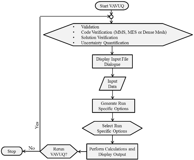
Figure 1: The general program operation can be conceptualized with a flow chart.

This section provides an overview of how quality control studies can be performed with the VAVUQ software.

Contents

• Starting VAVUQ
• Steps in Using VAVUQ to Evaluate a Model
• Determining Study Objective
• Viewing and Printing Results
• Getting and Using Help

Starting VAVUQ

A window appears when VAVUQ is launched. The window contains a toolbar, a dropdown menu with the different run options, and three buttons as shown in Fig. (2).

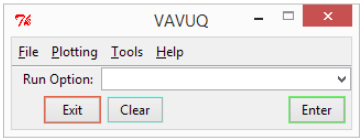
Figure 2: The initial VAVUQ window allows the selection of the main run options.

The toolbar allows the ability to access different program options. The “File” toolbar menu provides options for saving text output and nodal output in a spreadsheet format. The “Plotting” toolbar menu provides plotting options for both verification and validation. The “Tools” toolbar menu provides the option to focus on a specific region in a simulation domain. The “Help” toolbar menu provides options to view the program documentation and report bugs. When a run option is selected, the menus specific to the selected option will then populate the window and an open file dialogue will appear for selecting input data.

Steps for Model Evaluation with VAVUQ

Five main steps are required for using VAVUQ to quality control numerical approximations or validate a model.

• Determine the Study Objective (code verification, simulation verification, uncertainty quantification, model validation).
• Determine appropriate results or comparisons to use in the study.
• Prepare input data to be read by VAVUQ.
• Perform the desired calculations with VAVUQ.
• Visualize and interpret output data.

Determining Study Objective

The first step in using VAVUQ is to identify the study objective. For example, the goal can be to validate a mathematical model, verify the numerical approximations of a computer code, verify the simulation approximations applied to a specific system, or determine the discretization error uncertainty of a given numerical approximation. If validation is the goal, appropriate observational data needs to be obtained from a system and the approximations of that system have to be made with the model of interest. If code verification is the goal, an appropriately complex exact solution needs to be obtained or created to compare three numerical approximations to. For example, the exact solution can be obtained with an analytical solution, the Method of Manufactured Solutions, or a dense mesh. If simulation verification or discretization uncertainty quantification is the goal, at least three numerical simulations with refinements equal to or greater than 1.3 are required.

Preparing Input Data

VAVUQ can read various input file formats. VAVUQ is able to read data from .xlsx, .xls, .csv, .txt, .dat, and HDF5 files. The data has to be specifically arranged in order for VAVUQ to perform the calculations. For the spreadsheet file formats (.xls and .xlsx), the data for each discretization needs to be located in different tabs. Each tab needs to have unraveled matrices corresponding to the spatial coordinates and the simulation values in the first three columns as demonstrated in Table 1.

Table 1: Spreadsheet input files contain unraveled matrices with the spatial coordinates in the first two columns and the simulated parameter in the third column.

x1	y1	p1
x2	y2	p2
x3	y3	p3
⋮	⋮	⋮

The data arrangement for HDF5 files is similar to spreadsheet files with the exception that separate directories are used in the place of tabs. The directories with the data must be located adjacent to the root folder and be arranged in the format of Table 1. The data arrangement for .csv, .txt, and .dat files requires that the data is arranged successively in the format of Table 1 as demonstrated in Table 2.

Table 2: Data is entered sequentially for each simulation for .csv, .txt, and .dat files.

x1,1	y1,1	p1,1	x1,2	y1,2	p1,2	x1,3	y1,3	p1,3
x2,1	y2,1	p2,1	x2,2	y2,2	p2,2	x2,3	y2,3	p2,3
x3,1	y3,1	p3,1	x3,2	y3,2	p3,2	x3,3	y3,3	p3,3
⋮	⋮	⋮	⋮	⋮	⋮	⋮	⋮	⋮

Values in .txt and .dat files can be separated by both commas and tabs. The same number of separators needs to be used for every row in the input file. Exact solutions for the “Code Verification” option can be placed in each column to the right of the numerical simulation values as demonstrated in Table 3.

Table 3: Exact solutions can be placed in the columns immediately after simulation results.

x1,1	y1,1	p1,1	E1,1	x1,2	y1,2	p1,2	E1,2	x1,3	y1,3	p1,3	E1,3
x2,1	y2,1	p2,1	E2,1	x2,2	y2,2	p2,2	E2,2	x2,3	y2,3	p2,3	E2,3
x3,1	y3,1	p3,1	E3,1	x3,2	y3,2	p3,2	E3,2	x3,3	y3,3	p3,3	E3,3
⋮	⋮	⋮	⋮	⋮	⋮	⋮	⋮	⋮	⋮	⋮	⋮

The “Validation” option requires the numerical simulation values to be contained in the first tab of a spreadsheet and the benchmark values to be contained in the second tab of a spreadsheet.

Viewing and Printing Results

Once the user options are selected and “Enter” is pressed, interactive output graphs will appear. Graphs that are not interactive will be generated automatically in the working directory of VAVUQ. After graphs are displayed or generated, the program output is displayed in a textbox below the user input options. The contents of the textbox can be copied by selecting the text and then pressing <Ctrl + C> in Windows. The contents of the textbox can also be saved as a .txt file by accessing the save text dialogue in the file menu located on the toolbar. The plotted matrices can be saved to .xls spreadsheet files with the save matrices dialogue in the file menu located on the toolbar.

Getting and Using Help

VAVUQ offers multiple options to access help. The “Help” toolbar menu offers three different options to aid the user. The “About” option provides a brief description of VAVUQ and the program version. The “Documentation” option provides a link that opens the user’s Internet browser to the VAVUQ wiki page. The wiki page is the main and most up to date source of information pertaining to the VAVUQ program. The “Contribute/Report Bug” option allows the user to report potential issues with the program operation by directing the user to the project website. This option also allows the user to contribute code modifications or additions to the VAVUQ project. Another program feature to provide help to the user is an informative error message dialogue demonstrated in Fig. (3).

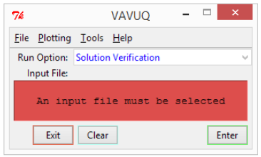
Figure 3: Error messages are displayed in a textbox with a red background below the user input.

The error dialogue can be used to direct the user to information that may be helpful to facilitate the program operation.

4 Example Applications

This section provides demonstrations of each major component of VAVUQ which includes Solution Verification, Code Verification, Uncertainty Quantification, and Validation. Images of the program operation are from a Windows 8 machine. The interface is designed to match the system theme of the user’s operating system. As a result, the program theme may change for different personal computers.

4.1 Solution Verification

Solution Verification can be used to calculate the observed order of accuracy for numerical simulations where an exact solution is unknown. Three numerical simulations with refinements equal to or greater than 1.3 are required. The Solution Verification run option can be selected from the dropdown menu in the dialogue when the program is first launched as shown in Fig. (4).

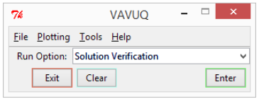
Figure 4: Solution Verification can be selected from the dropdown menu in the initial window.

A window will then be automatically generated that can be used to select an input file formatted appropriately for the selected run option as shown in Fig. (5).

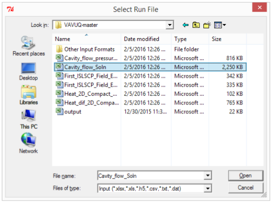
Figure 5: Input files can be selected graphically.

If the Solution Verification option is already selected due to a program restart, the “Enter” button can be pressed to generate the input file dialogue. The file can be selected by navigating to the directory containing the input file, selecting the file with a left mouse click, and then pressing the “Open” button. The main VAVUQ window will then be populated with the name of the selected input file and options specific to the Solution Verification run option. If an input file was selected by mistake, the “Clear” button can be used to return the user to the initial VAVUQ window. The Solution Verification option creates interpolation and output options as shown in Fig. (6).

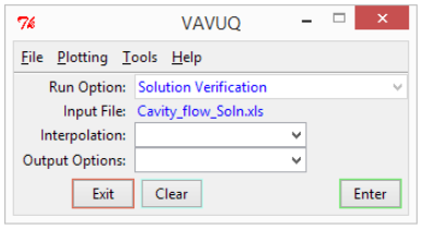
Figure 6: The Solution Verification allows interpolation and output option selections.

The interpolation options can be used to select different interpolation methods to relate simulation values. The output options provide the ability to generate figures and to generate output containing calculated norms. VAVUQ allows the ability to focus on specific areas within the simulation domain. This can be useful for large domains that may require excessive computational requirements for mesh interpolation. Generally areas with the greatest gradients are the most of interest for numerical simulations. The area of focus can be selected by checking the option “Cut Mesh” in the “Tools” menu on the toolbar. This will result in the generation of four input fields to provide the minimum and maximum desired extents in both coordinate directions as shown in Fig. (7).

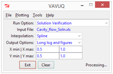
Figure 7: A specific area in the simulation domain can be selected for the computations.

After the selections are made and the “Enter” button is pressed, interactive plots will appear. Surface plots are the default plotting option. Other plot types can be selected under the “Plotting” toolbar menu. These plots allow the user to visualize the input data, interpolations, and program output. Each simulation is visualized as demonstrated in Fig. (8).

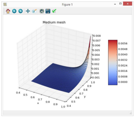
Figure 8: Input simulations are visualized.

Differences between refinements are visualized as demonstrated in Fig. (9).

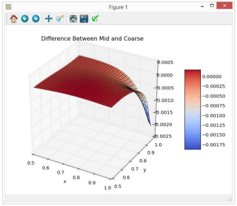
Figure 9: Solution differences due to successive refinements can be visualized.

The observed order of accuracy for each node can be visualized over an entire simulation domain as demonstrated in Fig. (10).

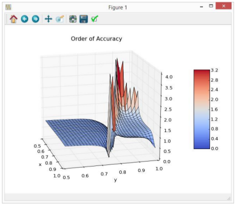
Figure 10: The point-wise order of accuracy can be visualized.

Observations of observed order of accuracy changes across a domain may provide insight about potential areas subject to modeling errors. The text output provided by VAVUQ includes copies of the user options, the directory and filename of the input file, whether the mesh is structured or unstructured, the ratios of the refinements, the norms of the simulation differences, the observed orders of accuracies calculated with the norms, and the median and average point-wise observed orders of accuracies. The calculations are made for the entire domain, the domain boundary, and the domain excluding the boundary. The text output is displayed below the user options and can be scrolled through with a scrollbar as demonstrated in Fig. (11).

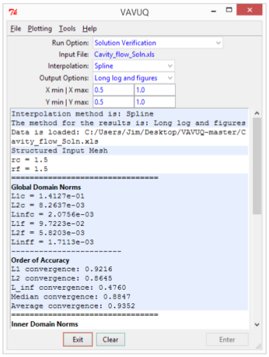
Figure 11: The text output can be analyzed when the calculations are finished.

At this point, the text can be saved to a .txt file by selecting “Save Output Text As..” from the “File” menu in the toolbar. Similarly, the point-wise results can be saved to a .xls spreadsheet by selecting “Save Output Meshes As..” from the “File” menu in the toolbar. The program can now be either exited or restarted. The user can exit the program by pressing the “Exit” button. The user can restart the program by pressing the “Clear” button.

4.2 Code Verification [MMS, MES or Dense Mesh]

Verification of the convergence of numerical approximations to a known exact solution can be used to assess the performance of a computer code. An exact solution and three numerical approximations with refinements greater than 1.3 are required for two approximations of the observed order of accuracy. The Verification run option can be selected from the dropdown menu in the dialogue when the program is first launched as demonstrated in Fig. (12).

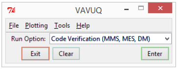
Figure 12: Verification can be selected in the dropdown menu in the initial window.

A dialogue will appear to select an input file when the verification run option is selected. After the input file is selected, additional options will appear. Options are similar to those produced for the Code Verification run option as demonstrated in Fig. (13).

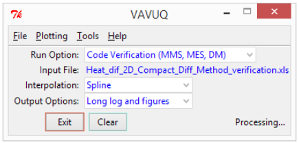
Figure 13: Verification specific options appear after an input file is selected.

If figures are selected in the “Output Options” dropdown menu, interactive plots will then be generated. Plots of the differences between each simulation and corresponding exact solution appear as demonstrated in Fig. (14).

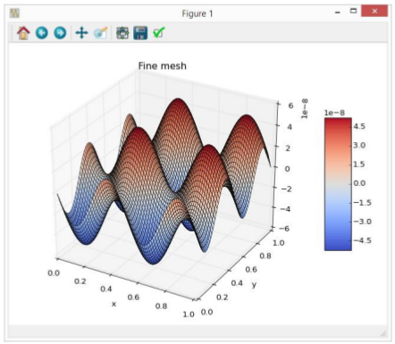
Figure 14: The input simulations are graphically presented.

Interpolations relating the calculations from the more refined meshes to the lesser refined meshes are then visualized as demonstrated in Fig. (15).

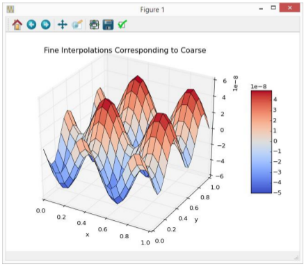
Figure 15: The interpolations are visualized.

The text results are then presented in the textbox below the user options as demonstrated in Fig. (16).

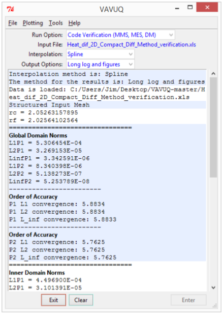
Figure 16: The verification text result can be viewed below the user options.

Text and mesh results can be saved to .txt and .xls spreadsheet files respectively with the “File” menu in the toolbar.

4.3 Uncertainty Quantification

Uncertainty Quantification can be used to estimate the influence of discretization errors. The estimation of these errors can provide insight on what appropriate discretizations may be for numerical simulations. Three numerical simulations are required for the Uncertainty Quantification option. Uncertainty Quantification can be selected from the “Run Options” dropdown menu as shown in Fig. (17).

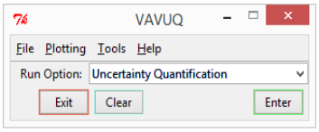
Figure 17: Uncertainty Quantification can be selected from the main window.

After an input file is selected, grid convergence confidence level options are generated in addition to interpolation and output options as shown in Fig. (18).

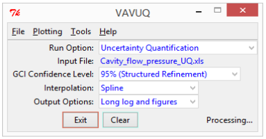
Figure 18: Different confidence levels can be selected for the grid convergence index calculations.

The different confidence levels or safety factors can be used to produce error bands with 95% and 99% confidence. Different safety factors need to be selected depending on whether the meshes are structured or unstructured. When the “Enter” button is pressed after the options have been selected, interactive plots will then be generated. The input simulation results are visualized as demonstrated in Fig. (19).

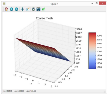
Figure 19: Results are visualized for the verification option.

The differences between the refinements are visualized as demonstrated in Fig. (20).

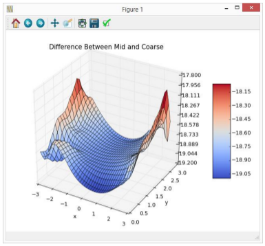
Figure 20: Differences between successive refinements are visualized.

The upper and lower bands of uncertainty are visualized as demonstrated in Fig. (21) & Fig. (22).

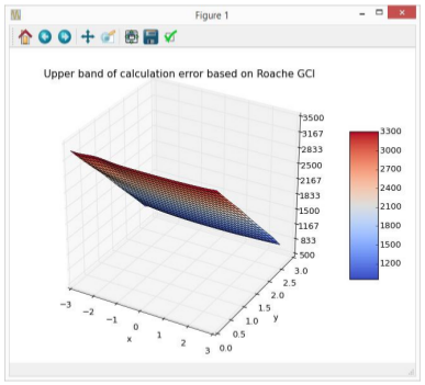
Figure 21: The upper band of uncertainty is visualized.

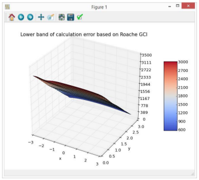
Figure 22: The lower band of uncertainty is visualized.

The textbox displays the norms of the differences between successive refinements as demonstrated in Fig. (23).

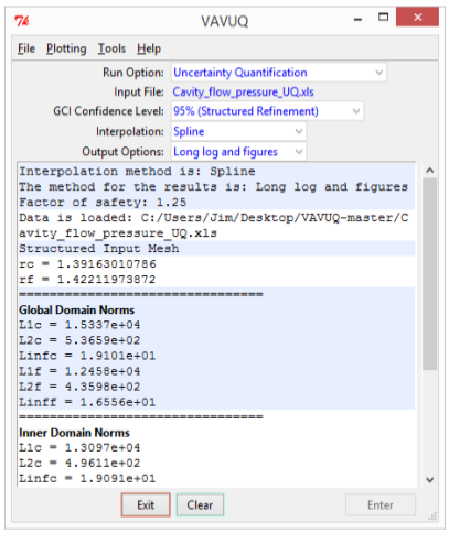
Figure 23: A textbox is displayed for the verification run.

The matrix calculations can be saved in a .xls spreadsheet file and the text can be saved in a .txt file with the options under the “File” toolbar menu.

4.4 Validation

VAVUQ can be used to calculate statistics useful for model validation. The validation option can be selected from the dropdown menu next to the “Run Option” label as shown in Fig. (24).

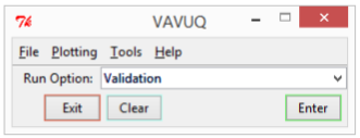
Figure 24: Validation can be selected from the main window.

A menu populates the window and an open-file dialogue will appear if either the “Enter” button is pressed or the “Enter” key is pressed on the user’s keyboard. After the validation input file is selected, the window will display the input file name along with options to produce a plot or generate statistics within a specified range of the data as shown in Fig. (25).

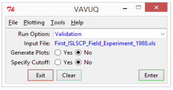
Figure 25: Validation specific options populate the main window when an input file is selected.

The input file can be an Excel spreadsheet with the first tab containing the numerical data and the second tab containing the benchmark data. Different plotting options can be selected from the “Plotting” toolbar menu under the “Validation” category. If the “Specify Cutoff” option is selected, two input fields will be generated to specify the percentage of the range of the benchmark data to generate statistics for. This option can be used to generate statistics for how well a model approximates a benchmark for a given portion of the range of the observed benchmark values as shown in Fig. (26).

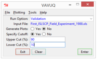
Figure 26: Validation calculations can be made for certain percentage cutoffs of the range of observed values.

The statistics will be generated and displayed in a textbox below the options after either the “Enter” button is pressed or the “Enter” key is pressed on the user’s keyboard as demonstrated in Fig. (27).

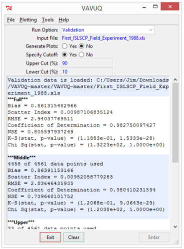
Figure 27: Validation calculation results are presented in a textbox below the user options.

The default plot option will produce a plot of the numerical versus the benchmark data as demonstrated in Fig. (28).

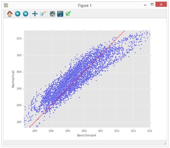
Figure 28: Plots are generated to visually validate models.

Contributing

If you would like to contribute code, you can do so through GitHub by forking the repository and sending a pull request.

Some of the priorities for future code releases include the following:

• Plugins to process data files specific to different simulation packages
• Additional analysis options useful for validation, verification, or uncertainty quantification

License

This program is free software: you can redistribute it and/or modify
it under the terms of the GNU General Public License as published by
the Free Software Foundation, either version 3 of the License, or
(at your option) any later version.

This program is distributed in the hope that it will be useful,
but WITHOUT ANY WARRANTY; without even the implied warranty of
MERCHANTABILITY or FITNESS FOR A PARTICULAR PURPOSE.  See the
GNU General Public License for more details.

You should have received a copy of the GNU General Public License
along with this program.  If not, see http://www.gnu.org/licenses.